The 2-SAT problem
The Boolean Satisfiability problem, also known as the SAT problem, is the problem of determining if there exists a set of values for the variables of a boolean expression so that it evaluates to TRUE. It has been proven to be NP-Complete, and is one of the most important and famous problems in Computer Science because it is the problem most used to prove other problems to belong in the complexity class NP, via reductions.
The SAT problem has lots of forms, one of them is the 2-SAT, in which the boolean expression is in Conjunctive Normal Form, i.e. a conjunction of clauses, and each of these clauses consist of 2 variables.
All known algorithms that solve the SAT are inefficient as they run in exponential time, and not much can be done to speed them up on a classical computer. However, by using a quantum computer and Grover’s algorithm, one can achieve an impressive speedup.
Grover’s algorithm
Grover’s search algorithm is a quantum algorithm that performs database search faster than its classical counterpart, by a polynomial factor. Concretely, if we were to search for example an unordered list of \( N \) elements (random access) looking for a particular element, we would have to look into every element of the list at the worst case, resulting in linear time of execution, \( \mathcal{O}(N) \). This scales exponentially relative to the bits of the input: \( N = 2^n \), so \(\mathcal{O}(2^n) \).
Grover’s can speed up the search in the general case using \( \mathcal{O}(\sqrt{N}) = \mathcal{O}(2^{\frac{n}{2}}) \) quantum gates, so it still exponential but faster by a quadratic factor, which is very useful.
What we’ll be doing
We’ll be solving a particular instance of the 2-SAT problem, by working our way through the construction of the quantum oracle needed for Grover’s and showing that it not only provides an answer, but it also finds all the solutions with only one Grover iteration.
The instance of the 2-SAT we’ll be solving is the following:
Given the boolean function \( f(a, b, c, d) = (a \lor \lnot b) \land (a \lor c) \land(\lnot b \lor d) \land(\lnot a \lor \lnot d) \), find if there exists an assignment of TRUE or FALSE to the variables \( a, b, c, d \) such that \( f(x) \) evaluates to TRUE.
We’ll be using IBM’s qiskit framework to simulate the quantum computer. IBM also gives us access to actual quantum computers where we can later upload the code and execute it there if we want.
The classical solution
By bruteforcing the expression, we can see the assignments that satisfy it are \( (a,b,c,d) = \{(0001), (0100), (0101), (1100)\} \):
from itertools import product

# reverse ordering due to the little endian bit-order in Qiskit
def f(d, c, b, a):
    return (a or not b) and (a or c) and (not b or d) and (not a or not d)

combs = list(product(*([[False, True]] * 4)))
sols = [f(*comb) for comb in combs]
for comb, sol in zip(combs, sols):
    print(f'{comb}\t->\t{sol}')
output:
(False, False, False, False) -> False
(False, False, False, True)  -> True
(False, False, True, False)  -> False
(False, False, True, True)   -> False
(False, True, False, False)  -> True
(False, True, False, True)   -> True
(False, True, True, False)   -> False
(False, True, True, True)    -> False
(True, False, False, False)  -> False
(True, False, False, True)   -> False
(True, False, True, False)   -> False
(True, False, True, True)    -> False
(True, True, False, False)   -> True
(True, True, False, True)    -> False
(True, True, True, False)    -> False
(True, True, True, True)     -> False
The quantum solution
First we need to implement the quantum oracle. To do this, it is convenient to re-write the expression as such:
$$ f = (a \lor \lnot b) \land (a \lor c) \land(\lnot b \lor d) \land(\lnot a \lor \lnot d) $$ $$ \Rightarrow f = (a + b’)(a + c)(b’ + d)(a’ + d’) $$ $$ \Rightarrow f = (a’b)’(a’c’)’(bd’)’(ad)’ $$
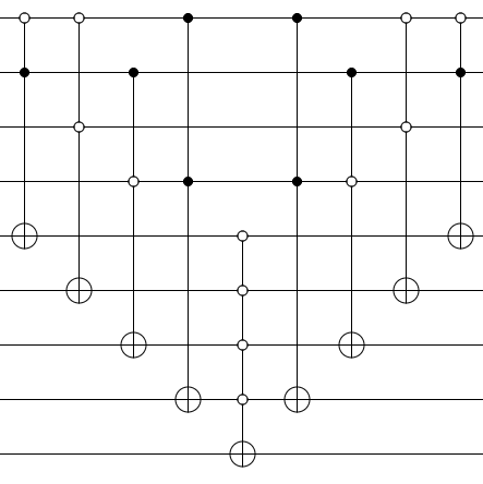
We need 4 qubits for the input, i.e. one qubit for each variable, and 4 ancilla qubits for each clause. Each clause will use one Toffoli gate, controled either low or high, depending on whether the variable in the expression is NOT-ed or not respectively. The Toffolis control an ancilla qubit each, and all the ancillas control a larger active-low C-NOT gate which controls Grover’s phase-cickback qubit \( | - \rangle \).
Now for the quantum oracle, we need to make it a unitary transformation, by definition. To do that, we just “mirror” the gates. The final output will be like this:
Now, we add the following:
- The Hadamard gates, to create a superposition of all the qubits
- The \( | - \rangle \) qubit
- Grover’s processing step
- Measurement step
Final circuit looks like this:
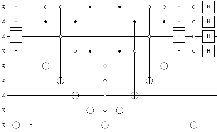
You can also find it here, simulated in Quirk.
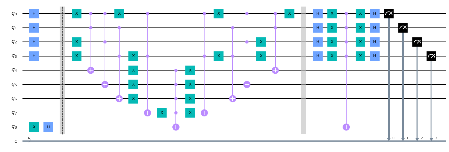
Now to implement it in qiskit, we add the following transformations:
- Active low control is an active high control surrounded with \( X \) gates.
- Two \( X \) gates next to each other cancel out because \( X^{2} = I \)
from lib import QuantumCircuit

qc = QuantumCircuit(9, 4)

# initialize output qubit to the "minus" state
qc.x(8)
qc.h(8)

# superpose
for i in range(4):
    qc.h(i)

qc.barrier()

# apply unitary
qc.x(0)
qc.x(2)
qc.mct([0, 1], 4)
qc.mct([0, 2], 5)
qc.x(3)
qc.x(0)
qc.mct([1, 3], 6)
qc.x(3)
qc.mct([0, 3], 7)

qc.x(4)
qc.x(5)
qc.x(6)
qc.x(7)
qc.mct([4, 5, 6, 7], 8)
qc.x(7)
qc.x(6)
qc.x(5)
qc.x(4)

qc.mct([0, 3], 7)
qc.x(3)
qc.mct([1, 3], 6)
qc.x(0)
qc.x(3)
qc.mct([0, 2], 5)
qc.mct([0, 1], 4)
qc.x(2)
qc.x(0)

qc.barrier()

# process (apply diffuser)
for i in range(4):
    qc.h(i)
    qc.x(i)

qc.mct(list(range(4)), 8)

for i in range(4):
    qc.x(i)
    qc.h(i)

# measure the 4 LSQs
for i in range(4):
    qc.measure(i, i)

_ = qc.draw(fold=-1, output='mpl')
Now we proceed to simulate the circuit:
from qiskit import QuantumCircuit

from qiskit import assemble, transpile, Aer
from qiskit.visualization import plot_histogram

def simulate(circuit, shots=2048, plot=True, ints=True, single=True):
    simulator = Aer.get_backend('qasm_simulator')
    transpiled_dj_circuit = transpile(circuit, simulator)
    qobj = assemble(transpiled_dj_circuit, shots=shots)
    results = simulator.run(qobj).result()
    answer = results.get_counts()
    if ints:
        answer = {int(k, 2): v for k, v in answer.items()}
    if plot:
        plot_histogram(answer)
    if single:
        answer = max(answer, key=answer.get)
    return answer


res = simulate(qc, single=False, plot=True, ints=False)
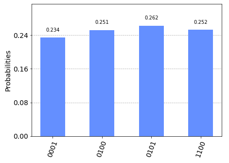
We can see that the probability amplitudes of the states that correspond to the \( k \) solutions are equal approximately to \( \frac{1}{k} \), and the rest are zero.
So indeed, with one run we get all the solutions at once. Very satisfying.
Concluding remarks
- This process can be easily generalized to solve 3-SAT or k-SAT.
- With qiskit, it is very easy to upload this and run it on a real quantum computer. It’d be fun.
- I am also sure there are ways to optimize this solution and use fewer gates.