Introduction
Volume rendering is a collection of methods to visualize volumes, which we often encounter in scientific, engineering, and biomedical domains.
Volume datasets are essentially sampled 3D scalar fields: \( f[m, n, k]: \mathbb{N^3} \rightarrow \mathbb{N} \). We refer to the pairs of 3D coordinates and their corresponding intensity values as Voxels (the 3D equivalent of pixels).
Volume rendering can be divided in three main categories:
- 2D visualization of slices of the volume, known as MPR (Multi-Planar Reconstruction)
- Indirect 3D visualization - Isosurfaces
- Direct 3D visualization known as DVR (Direct Volume Rendering)
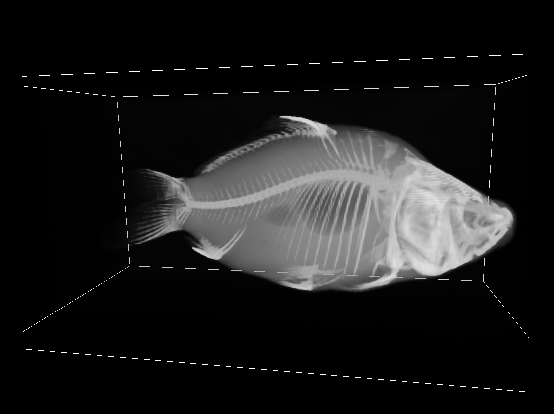
Let’s examine each category separately. All the examples presented below are generated on the 3D carp CT dataset, a popular volumetric dataset in the literature, often used as a benchmark in 3D volume rendering.
Multi-Planar Reconstruction/Reformatting (MPR)
This is a relatively simple method, where we generate a view alongside a plane perpendicular to the camera, through the center of the volume.
An example of this method can be seen below:
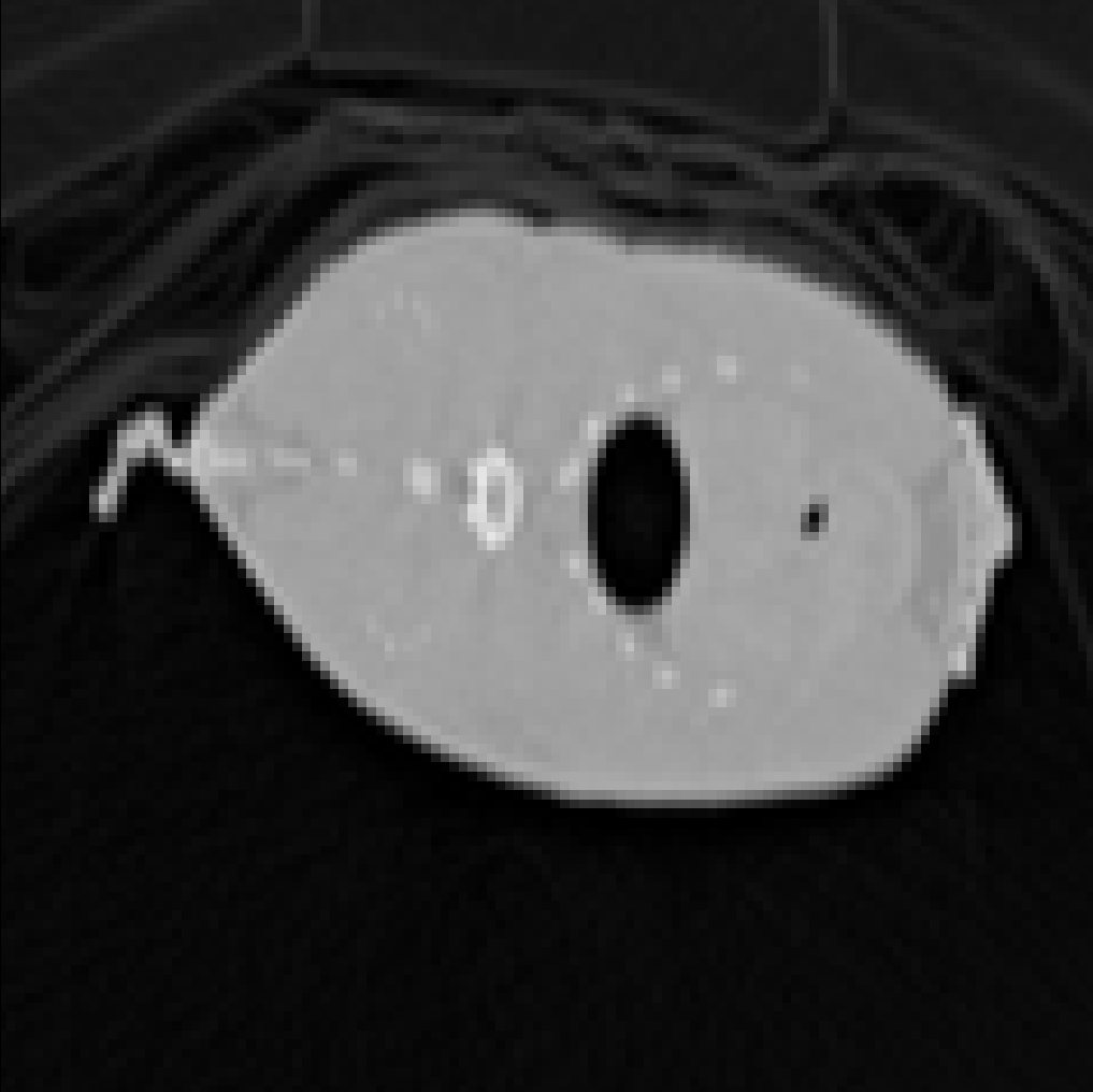
This image is the rendering of a “slice” of a carp (using Maximum Intensity Projection - we explain this in the DVR section). MPR is quite limiting because the view-plane has to pass through the center of the volume.
Direct Volume Rendering (DVR)
There exist two main methods to directly render voxels: ray-casting and voxel-projection. Ray-casting is most commonly used, and GPUs are great at it. It works as follows:
for each pixel of the screen:
    shoot a ray through the pixel and gather equidistant samples of the volume
    for each sample:
        calculate the position
        interpolate the intensity at the position
    calculate color along the ray by aggregating the intensities sampled
There are two ways to aggregate the intensities along a ray:
- Maximum Intensity Projection (MIP) - takes the maximum value out of all the samples
- Average Intensity Projection (X-ray like) - integrates all the values along the ray
Interpolation
When sampling along a ray, the samples almost always will not correspond directly to voxels of the volume. Hence, we need a way to estimate a value for the sample for the neighboring voxels.
The simplest way would be to just assign the value of the neighboring voxel. In fact, the first figure we saw above, in the MPR section, was generated this way. This is known as Nearest-Neighbor (NN) interpolation.
A more sophisticated approach would be to assume that the inter-sample values change linearly. This approach is known as Linear Interpolation and, since we operate with spatial values, Tri-Linear Interpolation - because we need to linearly interpolate along 3 dimensions.
Below is the same object as the one shown in the previous section, except it was rendered using Tri-Linear Interpolation to demonstrate the difference:
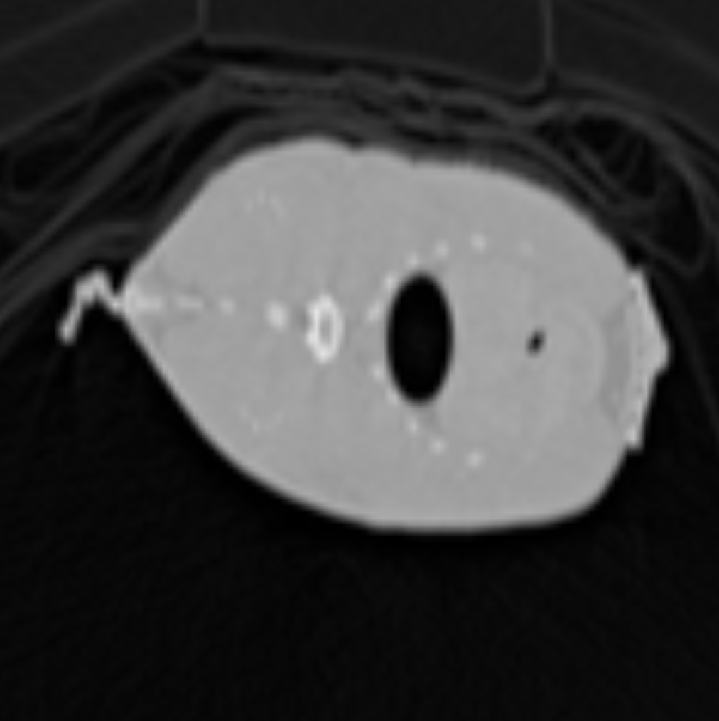
As we can see the edges are a lot smoother and the image overall is less “pixelated”.
Compositing - Emission-Absorption Model
With all the intensity projections we talked so far, we risk saturating the rendered image we get from the volume. This is why we use Compositing, an idea which simulates physical light transport through a semi-transparent medium that emits/absorbs/scatters light.
In this model, the accumulated color \(C’\) at position \(i\) is calculated recursively/iteratively as follows (back-to-front), using the opacity \(A_i\) at position \(i\):
\[ C^\prime_{i} = C_i + (1 - A_{i})C^\prime_{i+1} \]
Associated colors
In the formula above, the colors are not plain RGBA vectors but rather opacity-weighted RGBA vectors. These are called “Associated Colors”:
\[c_i = \begin{bmatrix}R_i\\G_i\\B_i\\A_i\end{bmatrix}, C_i = \begin{bmatrix} R_iA_i\\G_iA_i\\B_iA_i\\A_i \end{bmatrix}\]
Transfer functions
What if we want to visualize only specific intensity values of the volume? This would allow us to separate the volume into segments and make its various parts stand out, while also hiding other parts by setting their opacity to zero and making them transparent. For example, if our volume data are CT scans, we could specify the color of the bones to be different from the color of tissue.
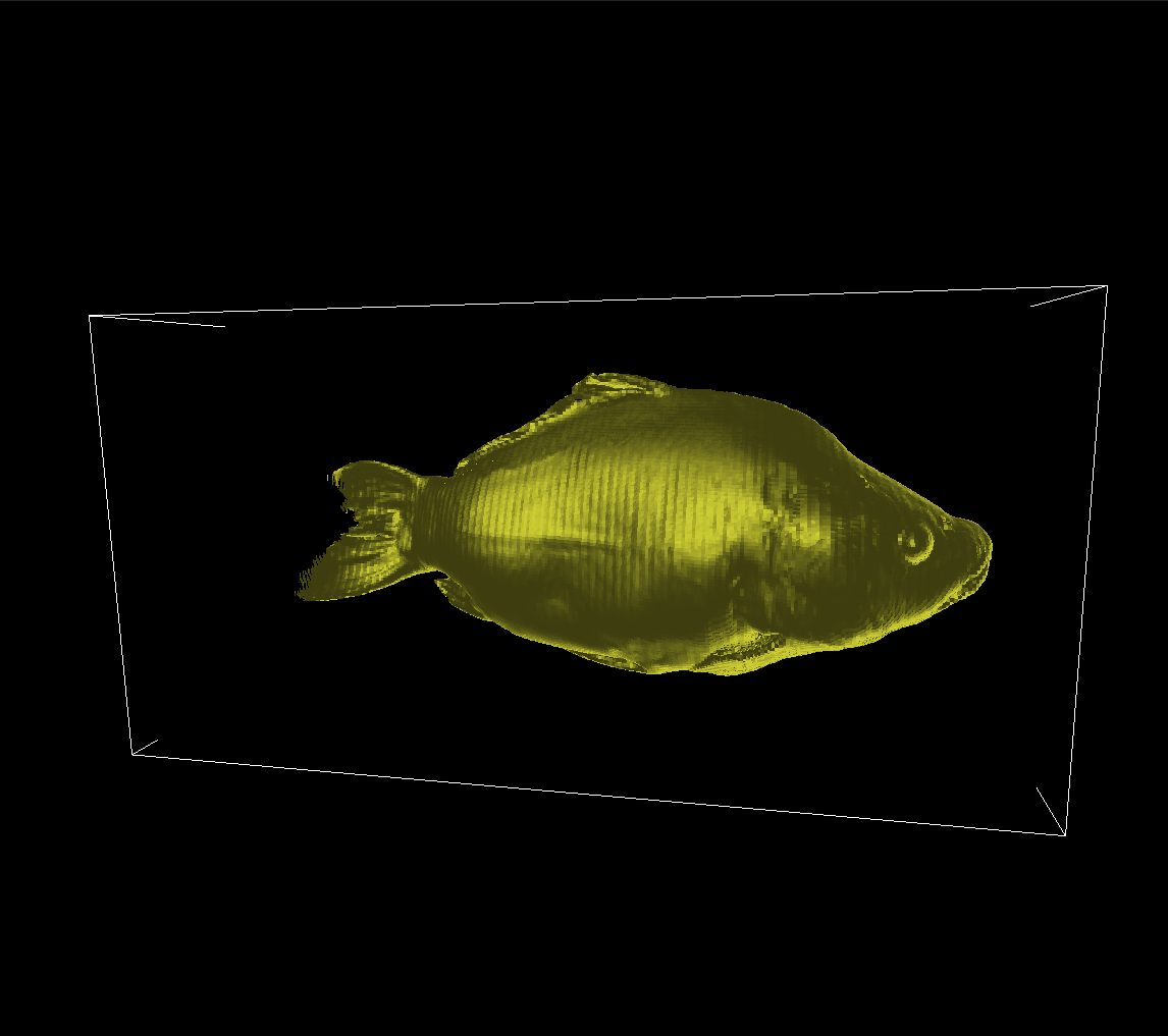
We can achieve this using Transfer Functions (TF). A TF maps the (interpolated) voxel intensity values from the volume into user-defined RGB/opacity values, before compositing. Let’s demonstrate this in the carp dataset. Using a monochromatic TF, we can get the following result:
If we map to RGB with a different TF that uses white for lower intensity values and yellow for higher ones:

Notice how the bones are visually separable from the tissue and the air bladder is also clearly visible.
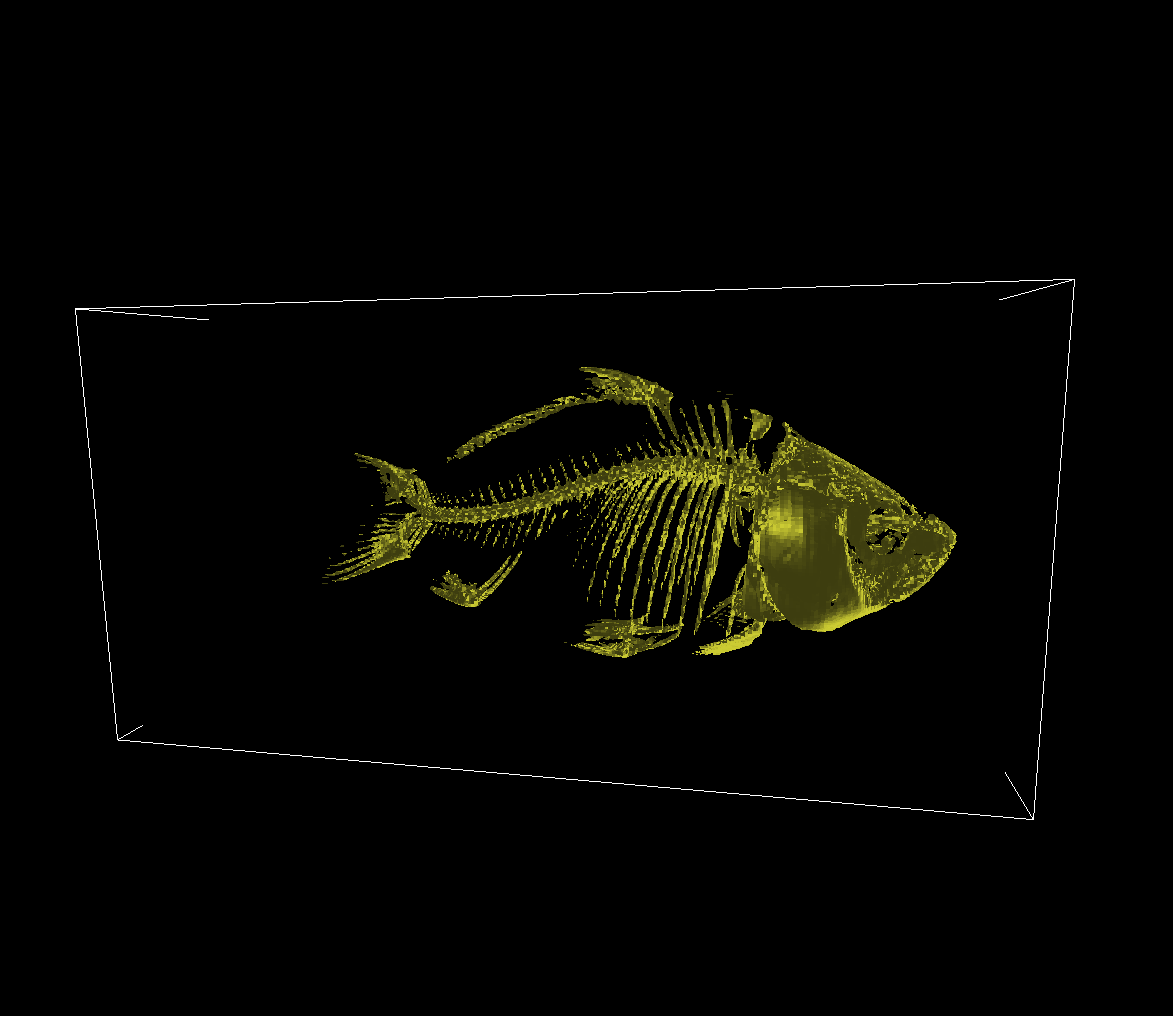
The TF can also be multi-dimensional, leveraging additional volume properties. Such a property could be the magnitude of the volume gradient, which may be used to capture “boundarieness”. This can help us better visualize surfaces, as demonstrated below:
Observe how clearly the internal surfaces are outlined in comparison to the previous methods.
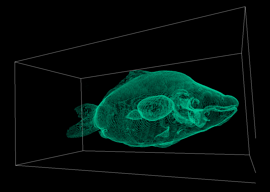
Indirect 3D visualization - Isosurfaces
Volume visualization using Isosurface Raycasting is simple: we sample the volume using rays like before i.e. we iterate along a line through the volume, except we stop when we encounter a value that is larger than a certain isovalue and we assign this value to our view pixel.
The result is conceptually and visually similar to a shadow cast by the volume onto our view:
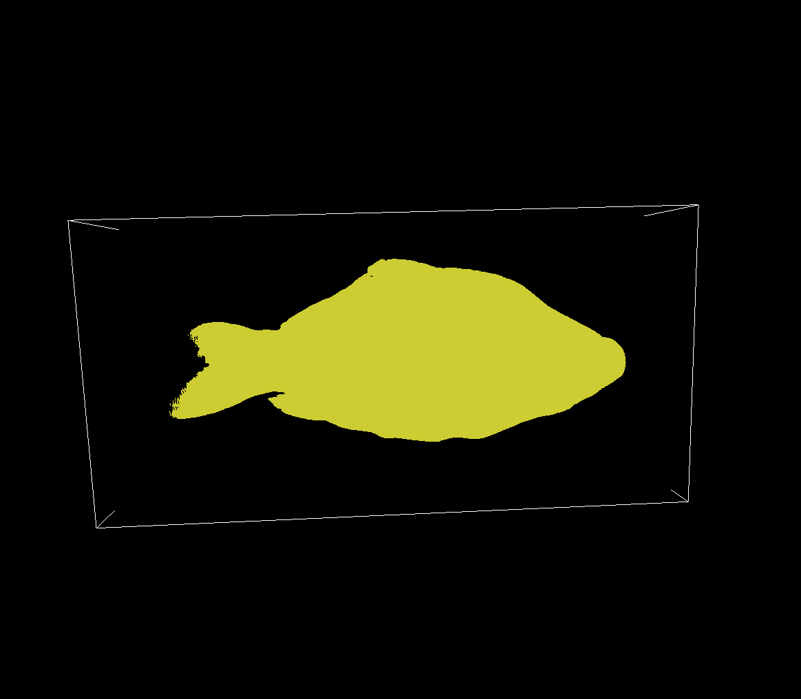
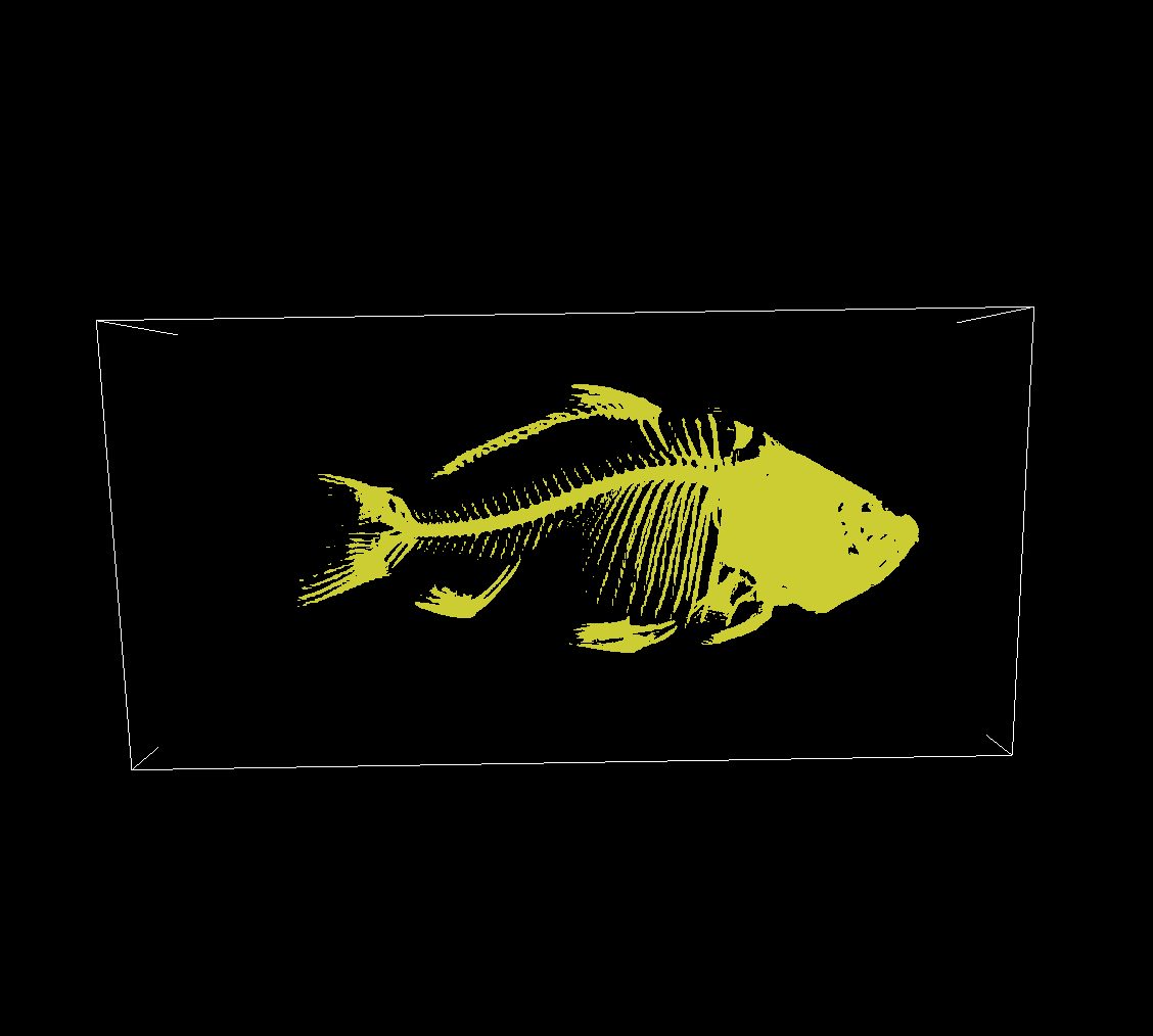
Setting a higher isovalue, we get an isosurface that outlines parts of the volume with higher intensities:
Bisection Algorithm
To better estimate the exact position of the isosurface, we can use binary search on the ray using the volumes’ intensity values. This is known as Bisection Algorithm and yields more accurate and more detailed surfaces.
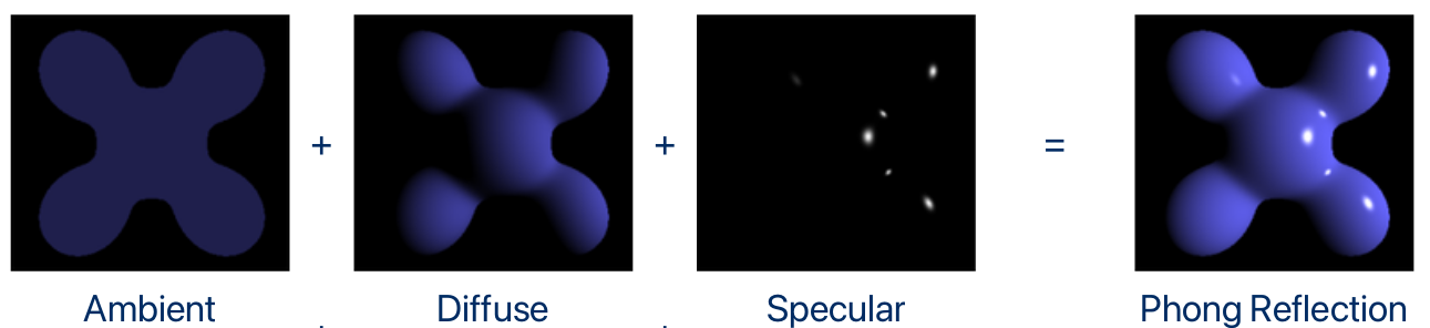
Phong shading
To actually visualize the surfaces as 3D, we need a shading model. The shading model will change the colors of the voxels of the isosurface to darker/lighter tones according to the volume gradients, camera position and light position to delineate the texture of the surface.
One of the most popular shading models is the Phong shading model. According to it, the final color of a point of a surface is equal to the sum of three different components: Ambient, Diffuse and Specular:
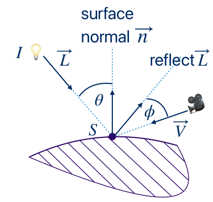
Formally, for a single light source:
\[ I_p = k_ai + k_d (\hat{L}\cdot \hat{n})i + k_s(\hat{R} \cdot \hat{V})^\alpha i \]
, where \( k_a, k_d, k_s, \alpha \) constants (describing the material), \(i\) the color of the voxel, \(\hat{L}\) the light vector and \(\hat{R}\) its reflection given by \( \hat{R} = 2(\hat{L}\cdot \hat{n})\hat{n} - \hat{L} \), \(\hat{n}\) (or \(\hat{G}\)) the normal vector of the surface on the point, and \( \hat{V} \) the camera position. Hats (\(\hat{}\)) denote normalized vectors.
The vectors are pictured in the figure below:
When used with compositing, shading is applied before compositing and after applying the TF.
By applying Phong shading and the Bisection Algorithm, we get the following results on our dataset’s isosurfaces, for the isovalues we used earlier:
Gradients
Until now we mentioned the volume gradients multiple times. How do we calulate them? The gradients can be calculated from the original data with central differences:
\[ G_x[i,j,k] = \frac{f[i+1,j,k] - f[i-1,j,k]}{2\Delta x} \] \[ G_y[i,j,k] = \frac{f[i,j+1,k] - f[i,j-1,k]}{2\Delta y} \] \[ G_z[i,j,k] = \frac{f[i,j,k+1] - f[i,j,k-1]}{2\Delta z} \]
\[ \vec{G} = \begin{bmatrix} G_x \\ G_y \\ G_z\end{bmatrix} \approx \vec{n} \]
They can then be cached/stored if enough memory/storage is available, in order to avoid recalculation every time which is computationally intensive.
Notes
I wrote this blogpost with the stuff I learned from the MSc course “Data Visualization” offered at TU Delft. It was a very interesting and well-organized course. The code for the Volume Visualization project (containing my implementations for the algorithms I used in this post) can be found here and here.